Using AWS Managed Grafana with Timestream for Observability: Writing Timestream Queries
In part two of a three-part series, we show you how to set up Timestream queries to measure and monitor AWS server performance.
In part one, we covered the basics of creating a Grafana workspace and configuring it to use a Timestream datasource for your server metrics. For the second installment, we’ll explore some basic Timestream queries and Grafana panels.
What is Timestream?
Timestream is a fast, scalable, and serverless time-series database service that makes it easier to store and analyze trillions of events per day.
We use Timestream to query our application servers and feed that data to Grafana for fancy dashboards, which allow us to measure and monitor important application server metrics like:
- Network activity,
- CPU usage,
- HTTP status codes,
- Database utilization, and
- Disk input/output performance (IOPs).

Step 1: Get Familiar with the Timestream Query Editor
You should use the AWS console query editor to explore your Timestream tables and craft some basic queries. The error output is particularly useful for debugging query syntax.
To get started with a query, choose the Preview Data option from the Query Editor in the Timestream console. Navigate to your Timestream ⭢ Query editor page, and select your database from the dropdown box. On the left hand side click the ellipsis next to a table and select Preview data. That will populate the query editor with a basic SELECT statement for you.
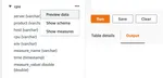
Clicking Run on the above panel will return 10 rows of data from the CPU table in the my-timestream-db Timestream database. From here you can modify a query to suit your needs - see the the query language reference for Timestream for more.
Step 2: Modify Timestream Queries for Grafana Panels
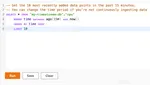
When altering your console-generated queries for use in Grafana graph panels, use Grafana variables. For instance, you should use something like the following in your WHERE clause:
WHERE time between from_iso8601_timestamp('${__from:date:iso}')
               and from_iso8601_timestamp('${__to:date:iso}')
This step will limit your data collection to the current time window for the dashboard.
Step 3: Step 3: Add a CPU Panel
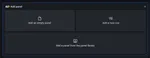
Click the Add panel button on your dashboard, and select Add an empty panel.
Select the appropriate Timestream region in the Data source dropdown box, and add the following query where $server matches a server name you have tagged in your Telegraf output:
SELECT server, BIN(time, 60s) AS time,
   ROUND(AVG(measure_value::double), 2) AS avg_usage_user
FROM "my-timestream-database".cpu
WHERE measure_name = 'usage_user'
   AND server = '$server'
   AND time between from_iso8601_timestamp('${__from:date:iso}') and from_iso8601_timestamp('${__to:date:iso}')
GROUP BY server, BIN(time, 60s)
ORDER BY time ASC
Note: you can replace $server in the query above with text, or use it as a Grafana variable on your dashboard.
Pro Tip: Use the Timestream Macros
Timestream’s query editor accepts a number of macros, including:
$_databaseto specify the selected database,$_tableto specify the table, and$_measureto specify the measure.
We’ve found these very useful in building our panels - and you probably will, too.
Click the Graph refresh button and you’ll get a preview of the data:
To provide more context to your graph, we suggest to:
- Add a title on the right hand side under Panel options and click the Save button.
- Change the Unit under Standard Options to Percent (0-100).
- Optionally, add another query by clicking the +Query button, and paste in the query we just used, but with
usage_systeminstead ofusage_user. - Under Graph Styles, enable the Stacked mode.
Step 4: Add an HTTP Status Panel
If you’re using a Telegraf plugin to process your web server logs, you can make a panel that displays your traffic by HTTP status class using a variation on the following query.
Create a new panel, then add the query below, where web_log is the table your web logs are in. You may need to change the measure_name to match the column where your status codes are logged.
WITH binned_timeseries AS (
SELECT BIN(time, 60s) AS time,
COUNT(time) AS status_count
FROM "my-timestream-db".web_log
WHERE measure_name = 'status'
AND measure_value::bigint > 199
AND measure_value::bigint < 300
AND server = $server
AND time between from_iso8601_timestamp('${__from:date:iso}') and from_iso8601_timestamp('${__to:date:iso}')
GROUP BY BIN(time, 60s)
ORDER BY time ASC)
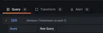
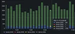
SELECT CREATE_TIME_SERIES(time, status_count) FROM binned_timeseriesClick on the Panel name, which should default to A, and rename it to ‘2XX’.
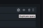
Use the Duplicate query button to add three more panels. Change the ranges on the WHERE clause to match the 300-399, 400-499, and > 500 ranges. Modify the query names to 3XX, 4XX, and 5XX to match the ranges.
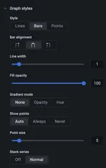
Under Graph Styles, change the Style to Bars, and set Stack series to Normal.
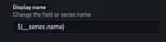
Set the Display name to ${__series.name} - this will add the name for the query in the panel legend.
Define the color scheme for the panels to differentiate them (and to prevent the colors from being auto-assigned). We went with green for 200 codes, blue for 300 codes, and orange for 400 codes.
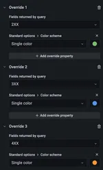
Finally, click on Save in the upper right hand corner.
Step 4: Add a Delta Query
Some stats are only available as counters that reset at system boot, when an application is started, or under various other limited conditions (for example, the linux networking stats you see when running netstat -s). Often, to make use of the data for graphs for alerting, we need to measure the changes of those values in a given time window.
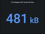
Let’s say you’re using the PostgreSQL input plugin to collect information from your Postgres database, and you’re interested in your average tempfile size. The two counters, temp_files and temp_bytes, represent the total number of temporary files and volume of temporary data in bytes since the last statistics reset.
One way to display your average temp file size would be to simply create a stat panel that divides temp_bytes by temp_files. That will give you the overall average. But, if you’re looking to see changes in the average temp files size over time there’s a better way: use the MIN() and MAX() functions to calculate the change in a given time window.
To add a stat panel, create a new panel and then set the type to Stat in the upper right hand corner drop box.

The query below first calculates the changes for temp_bytes and temp_files by subtracting the MIN() value from the MAX() value from our time window, before dividing them for the average. The NULLIF()'s are there to stop any dividing by zero nonsense.
SELECT NULLIF(temp_bytes, 0) / NULLIF(temp_files, 0) FROM (
 SELECT MAX(measure_value::bigint) - MIN(measure_value::bigint) AS temp_bytes
   FROM "my-timestream-db"."postgresql"
   WHERE measure_name = 'temp_bytes'
     AND db = '${server}'
     AND time between from_iso8601_timestamp('${__from:date:iso}') and from_iso8601_timestamp('${__to:date:iso}')),
 (  SELECT MAX(measure_value::bigint) - MIN(measure_value::bigint) AS temp_files
   FROM "my-timestream-db"."postgresql"
   WHERE measure_name = 'temp_files'
     AND db = '${server}'
     AND time between from_iso8601_timestamp('${__from:date:iso}') and from_iso8601_timestamp('${__to:date:iso}'))
Here’s our completed stat panel in all its glory.
Pro Tip: Use Intervals to Fix Slow Loading or Failed Panels
When adjusting the time window for a dashboard to cover a period longer than a couple of days, you may find that some Grafana panels are taking a long time to load or fail to load. When that happens, it’s likely that you’re loading and graphing too many data points.
For example, if you have a static interval of one minute, and are trying to view a month’s worth of data, you need to load 43,200 values for each metric - and it’s unlikely you need a resolution of 1 minute to make sense of that data across a month. Setting the $__interval value for your queries will allow the resolution to match the dashboard appropriately, reducing the number of data points, and speeding up load time considerably.
Step 5: Use Delta Queries with Window Functions
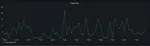
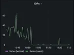
What if you want to show changes as they happen over a time window, instead of in total across the whole thing? One way to do it is by using a window function, and Timestream supports several. The query below uses the LAG() function to calculate changes over time by subtracting previous from current values.
SELECT server, BIN(time, 60s) AS time, SUM(delta)
FROM
   (SELECT server, name, time,
       ( measure_value::bigint - LAG(measure_value::bigint)
  OVER (ORDER BY name, time ASC)) / 60 AS delta
    	  FROM "my-timestream-db"."diskio"
   	  WHERE measure_name = 'writes'
            AND server = '${server}'
            AND time between from_iso8601_timestamp('${__from:date:iso}') and
                             from_iso8601_timestamp('${__to:date:iso}')
        )
GROUP BY server, BIN(time, 60s)
ORDER BY time ASC
OFFSET 1
Here’s an example of a panel showing read and write IO from the diskio plugin.
Quick Recap
In this guide, we:
- Covered the basics of using the Timestream Query Editor,
- Modified some Timestream Queries for Grafana panels, and
- Added a few panels to track our data, including examples with delta queries.
Coming up in part 3, we’ll show you how to monitor scheduled tasks with Grafana and use graph annotations the Network Ninja way.
If you’d like to work on cool stuff like this with us, check out our 100% remote (work from home) job openings.
Date
Reading Time
17 minutes
Next article
Using AWS Managed Grafana with Timestream for Observability: Scheduled Tasks & Graph AnnotationsCategory
Are you a developer? We’re hiring! Join our team of thoughtful, talented people.